9. About background modelling (superflatting, defringing, near-IR sky models)

This section provides some important information about background modelling. Its content must be understood in order to perform data reduction correctly. The THELI documentation makes use of the nomenclature and concepts presented here.

In particular in wide-field imaging, and/or observations at longer wavelengths, images will not appear flat after flat-fielding. Reasons are manifold:

• improper illumination or size of the domeflat screen
• scattered light in the dome while taking twilight flat fields
• moonlight
• differential airglow at higher airmass
• variable sky background (in particular in the near-infrared)
• sky concentration (reflection between CCD and corrector lenses)
• fringing
• pixel scale variations
• etc

Apart from fringing, these effects show up as low frequency spatial variations of the background level. Amplitudes may reach or exceed 10% of the background level. A background model is required to correct for these effects.

9.1. Airglow

9.1.1. Temporal variations

The higher atmosphere contains OH^– molecules which are excited during daytime and slowly decay at night. The spectrum of this airglow is characterised by clusters of numerous emission lines, starting at around 600nm and beyond.

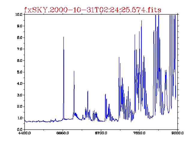
Movie of optical airglow spectra taken with UVES/VLT (credit: Ferdinando Patat, ESO)

The airglow’s intensity, temporal and spatial variability increase significantly with wavelength, dominating the near-IR sky:

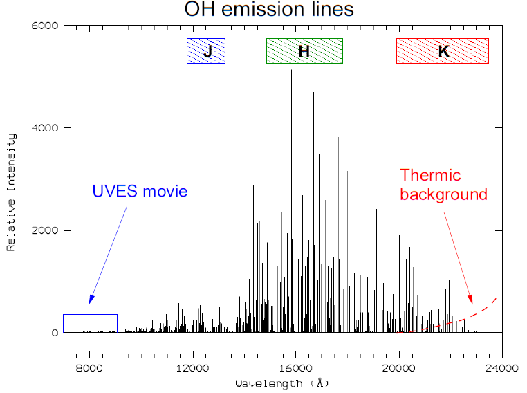
The spectral range covered by the movie of the optical airglow is indicated by the small blue box to the lower left. Notice how much brighter the near-IR sky is.

9.1.2. Fringing

CCDs are made of silicon, which becomes transparent with increasing wavelength, starting at around 700nm. In back-illuminated, thinned CCDs airglow can cause internal reflections leading to a characteristic interference pattern in the background of an image, known as fringing. The pattern itself depends mainly on the thickness of the CCD and is thus essentially unchanged over the lifetime of the detector. However, the amplitude of the fringing pattern varies as the airglow spectrum at a given position on the sky changes with time. Fringing is also present in near-IR detectors.

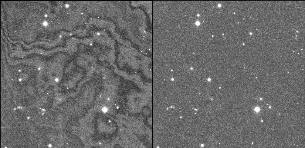
Fringing in I-band before and after correction.

In R-band this is usually not very critical and one fringe model will suffice for an entire night. In I-band things are more critical and in the worst case a new fringing model is needed every 30 minutes. In the near-IR the sky changes over time scales of minutes, and on angular scales of arcminutes, requiring new background models about every 5-30 minutes. In the mid-IR we talk about seconds. Fringing is less important in these cases, more problematic are the sky background variations themselves:

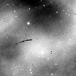
This is a movie of the near-IR H-band airglow over 1.5 hours. The field of view is 9 degrees, 1 second in the movie corresponds to 7 minutes real time. The mean background level has already been removed, shown are only the variations around the mean. Hence reality is even worse than depicted here. (Credit: 2MASS wide field airglow experiment).

9.2. How to create a background model

A background model can be created from a set of dithered exposures of a non-crowded (or empty) field. The dither pattern has to be significantly larger than the largest object in the field. Extended objects must be absent or otherwise the correction image will be wrong.

THELI applies several steps in order to create a background model. First, all objects in an exposure are detected and masked, such their flux will not bias the result. The masked images are rescaled to the same mode and then median combined. If all goes well, the background model contains only background signal. This can be a pretty featureless image, or it can show significant large-scale variations and/or small-scale fringing.

The high-frequency fringing component can be extracted from the background model by smoothing the latter with a large (several hundred pixels wide) kernel, and subtract the smoothed image from the unsmoothed model. This is often used for optical data to separate a multiplicative illumination correction from the additive fringing component. In the near-IR, the original background model would be subtracted from the data.

9.2.1. Static background models

A static background model is created from a fixed set of exposures, and applied to all images in the data set. This will only work reliably well if the background is stable during the night or at least over longer stretches of time.

The sky becomes more unstable with increasing wavelength. In R-band the fringing is usually low and varies slowly, thus one static model (for fringe correction) usually suffices for the entire night. For the I-band this is also possible if conditions were stable, or if target observations did not extend over more than 30-60 minutes in bad conditions.

9.2.2. Dynamic background models

In the near-IR, static models can only be used if target observations do not exceed 5-30 minutes. Otherwise a dynamic background model is required, i.e. the correction image is calculated from a number of contemporal exposures. One would like to make this window as large as possible in order to improve the S/N in the correction image, but it has to be kept as small as necessary to still properly sample the temporal sky variations. This can require some trial- and error in data reduction. Typical window sizes are 6-10, i.e. these many images closest in time to the exposure being corrected are used to create the model. The computational overhead for a dynamic model is larger than for a static model.

9.3. Superflat or sky background model?

Background variations can have additive or multiplicate causes, such as scattered light (additive) or an incorrect flat field (multiplicative; which might be caused by an additive effect, such as scattered light or sky concentration).

A good background model will always result in a flat image, no matter how it is applied. However, if you accidentally correct a multiplicative effect by subtraction, then the photometric zeropoint will no longer be constant across the field. Likewise, an exposure with constant zeropoint may not have a constant sky background, which must be subtracted afterwards. If the goal is to achieve a flat background and photometry isn’t important for your work, then you most likely do not care about all of this. However, if consistent photometry matters, you are in for a good deal of trouble, as multiplicative and additive components are hard to distinguish, in particular when they occur simultaneously.

• Multiplicative character: The background model falls in this category if the flatfield wasn’t working correctly. This is very often the case with wide field imagers, leaving residuals on the level of 1-2 percent. Reasons can be manifold, e.g. the flat screen is insufficiently illuminated or too small, sky concentration, or else. In this case the data must be divided.
• Additive character: Even if the flatfield itself is perfectly fine, it happens that the flatfielded data still exhibits significant background variations. In the optical this is usually the case due to scattered light finding its way onto the detector. In the near-infrared, the dominant component is the sky background itself (airglow). In these cases the background model has to be subtracted from the data.

If one erroneously subtracts a background model instead of dividing by it, or vice versa, the resulting background will still be perfectly flat, but the photometric zeropoint will not be constant anymore (variations of up to 10% are not uncommon).

Interpreting the background structures sometimes helps to identify the correct approach, but it can be misleading. For example, flat field effects are often radially symmetric whereas scattered light can cause one side of the image to be brighter than the other if caused e.g. by moonlight. It may also be symmetric, e.g. when caused by light being reflected from the detector to a field corrector lens, and from there back again to the detector. In such cases one would have to correct the flat field for scattered light first, but for the observer this is usually not possible as it requires extensive testing at the telescope.

If both additive and multiplicative effects are mixed, there is only way to fully correct for it: one must compare the data with photometric reference data from the same field and in this way establish a map of the zeropoint variations, from which a (multiplicative) correction image can be calculated. This requires a comparatively high density of reference objects and a good photometric catalogue of your field in the same filter (if your field is covered e.g. by SDSS, then you have a good chance to correct for it). Alternatively, you could observe an external standard star field with excessive dithering and calculate a correction image which you apply to your data, assuming that the effect is stable. After this multiplicative correction, residual background variations can be modelled and subtracted individually.