10. BACKGROUND

This section deals with correction of background variations. This can either be superflatting, defringing or subtraction of a background model. For mid-IR data a suitable chop-nod sky subtraction is offered. Lastly, in order to remove typical effects such as reset anomalies in near-IR cameras, a collapse correction can be performed.

If you are unfamiliar with background models, then please read this background information first.

10.1. Spread sequence (NIR)

LIRIS@WHT is the only near-IR detector I’m aware of that needs this treatment. So most of you can simply skip this section. Nevertheless, I’m going in some details in case it crops up in other instruments (likely using older HAWAII-1 arrays).

10.1.1. Resetting and image equilibrium

Near-IR detectors have very different properties than the CCDs used in optical instruments. While they are not exposed, they are continuously resetted and rapidly reach a resetting equilibrium. On the other hand, when a series of exposures is made, the detector reaches an imaging equilibrium. I have made up these two terms myself, so if you know a more precise or commonly used wording, then please let me know.

If you have dithered observations with LIRIS@WHT, and a series of e.g. 10 exposures was taken per dither point, then the detector will have reached the imaging equilibrium with the third exposure. All subsequent images will have the same (instrumental) background. While the telescope acquires the next dither position, the detector goes into the resetting equilibrium again and thus is in the same state as when you started the exposure series at the first dither position. Therefore, the image backgrounds are the same for the i-th exposures in the n-th sequence (apart from slower sky background variations). The consequence is that the background modelling has to be done separately for these exposures. This script sorts the data in according directories where it is then processed automatically in the right manner.

Warning

It is essential that you do not mix sequences with different lengths in the SCIENCE directory. THELI assumes that only complete sequences of the same length are present.

10.1.2. Example

You have 12 images per dither point. From subtracting one image from the next in the sequence, you found out that the detector settled into its imaging equilibrium starting with the third exposure. You would then enter 3 into the field # groups, and 12 into the one labelled Length.

The script will create three directories next to the SCIENCE directory, and redistribute the exposures in the following manner:

* SCIENCE_S1: exposures 1, 13, 25, ...
* SCIENCE_S2: exposures 2, 14, 26, ...
* SCIENCE_S3: exposures 3-12, 15-24, 27-36, ...

The background modelling must be done separately for each of these directories. THELI will do this automatically for all SCIENCE_Si directories and, if applicable, SKY_Si directories. You do not have to make any changes in the directory tree defined in the Initialise section.

All other processing tasks do not (and do not have to) loop over the SCIENCE_Si directories. THELI will know that it has to do this loop if the Spread sequence (NIR) task has either been executed, or is activated.

After the background has been corrected, you merge the images again into the previous SCIENCE directory. This is done further below (see the Merge sequence (NIR) task). SKY fields are processed automatically after the SCIENCE data have been dealt with.

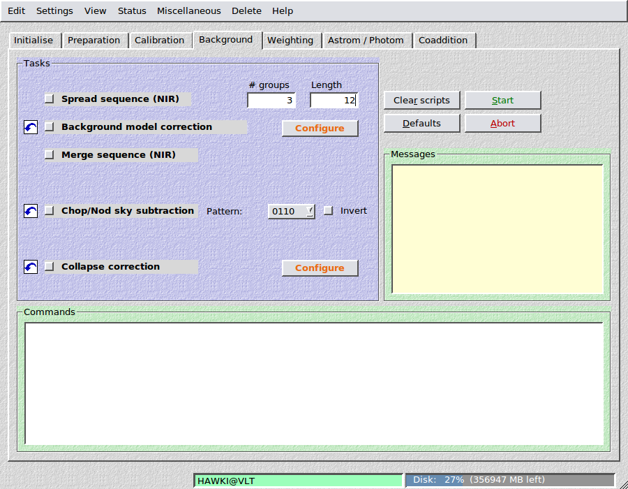
10.2. Background model correction

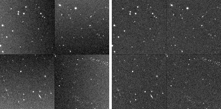
This task will create the background model, and apply it in a variety of ways, depending on whether you process optical or near-IR data. The resulting images may have suitably flat background after a first pass, but faint and unmasked haloes will have contributed to the background model and then show up as darker patches, reflecting the dither pattern (see the left panel below):

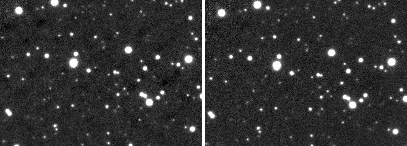
Use the two-pass mode to correct for this effect (see the parameter choices below). The improved result can be seen in the right panel above. For your reference, THELI will keep the images with the single-pass subtraction in a OFCB_IMAGES_1PASS directory.

Filename extension: Images will have the character B appended to their filenames, e.g.

NGC1234_1OFCB.fits

10.2.1. Parameters

Background modelling in THELI is highly configurable, to match the different demands and characteristics optical and near-IR data may have. Four main parameter groups are available to control this task, described in detail below.

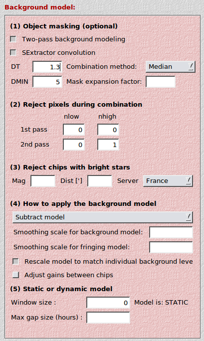
1. Object masking (optional):

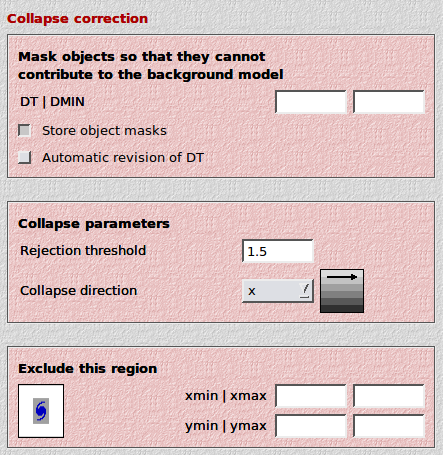
   • Two-pass background modeling: If activated, then THELI will create a median-combined (without object detection) to remove the bulk of the background signal. A refined step includes object masking (using e.g. DT=1.5, DMIN=10), which are applied before combining the OFC images once more for the background model.
   • SExtractor convolution: THELI will do a SExtractor convolution prior to object detection. However, this may increase the footprint of hot pixels. If you have lots of hot pixels, you may consider switching this setting off.
   • DT: This is the SExtractor detection threshold per pixel, given in units of sigma of the sky background noise. If you leave it empty, no object masking will take place.
   • DMIN: The minimum number of connected pixels above the detection threshold making up an object. The smaller DT and DMIN, the fainter the objects masked. If you leave DMIN empty, no object masking will take place.
   • Median/mean: The method used for combining images. The median delivers a more stable result for a small number of stacked images, whereas the mean has lower noise when more images are stacked, but is susceptible to outliers. The default setting is median.
   • Filter: If a lot of hot pixels are present in the data, then consider to switch off this option. Filtering increases the footprint of a pixel and thus the fraction of the masked area can become unacceptably large, e.g. for some particularly bad HAWAII-2 arrays.
   • Mask expansion factor: The SExtractor isophotal ellipse is scaled by this number. If set to a number larger (smaller) than 3, the isophotal ellipse will become larger (smaller) than the extent of the detection. This may become necessary if extended low surface brightness objects are present whose extent cannot be detected directly in a single exposure. If you notice that diffuse objects are surrounded by darker halos in the coadded image (or individual exposures), then you should consider setting this factor to a higher value, such as 6-10, or even more. Note, however, that this requires sufficiently large dithering to retain a good number of sky pixels. Otherwise just leave it empty.

   The final mask images are stored in a separate MASK_IMAGES directory where they are available for inspection. If masking is switched off, then you will simply find links to the unmasked images from which the background model will be created. If masking takes place, then you should inspect the mask images to make sure that masking is not too aggressive. The latter would be the case if not only objects, but also sky features are masked.

2. Reject pixels from the stack:

   This can be adjusted separately in case a two-pass approach is chosen.

   • nlow: The number of lowest pixels in the stack to be rejected. Default: 0
   • nhigh: The number of highest pixels in the stack to be rejected. Default: 1. Therefore, even if you decided to not do an object detection (leaving DT and DMIN empty), you will get a rather clean background model.

3. Reject chips with bright stars:

   • Mag: Chips with stars brighter than this magnitude will not be included in the background calculation. A bright star catalog is retrieved from one of the online CDS servers.
   • Dist [‘]: A bright star must be at least this many minutes outside a chip for the chip to be considered good for background modeling (thinking of large PSF halos).

3. How to apply the background model:

   This is the most important part of the background modelling process. Here you decide how the model is applied. Whatever suits your optical or near-IR data best. Note that individual images may still present some background residuals afterwards, which have to be removed using sky subtraction. The following options and settings are available:

   • Subtract model: This is your choice for near-IR data. The background model will by default be rescaled (see below) to match the illumination of the individual images, and then subtracted. Possible fringes in the data are removed as well.
   • Divide model: This corresponds to classical superflatting, often used for optical data. Note that background gradients in optical data are often caused by differential airglow or scattered light, and should therefore be subtracted, not divided.
   • Subtract fringes: In this mode the background model will be smoothed with a large kernel (usually several 100 pixels, see below), resulting in an illumination correction (superflat). The smoothed model is subtracted from the unsmoothed model, yielding the desired fringing model with the higher frequency variations. The fringing model will be rescaled to match the variations in the science image, and subtracted. This mode would be applied to optical data when fringe correction is desired, but no superflatting.
   • Divide smoothed model, subtract fringes: Same as the previous, but in addition to defringing the science image gets divided by the normalised illumination correction, i.e. a superflat is applied.
   • Create masks only, do not apply them: If this option is chosen, only the masks will be created. Change the object detection parameters DT and DMIN and rerun the task until you are satisfied, then choose one of the four other modes.

   These modes can be fine-tuned by the following settings:

   • Smoothing scale for the background model: This would be a several 100 pixel wide kernel to smooth the background model. Required if you want to subtract fringes, or divide by a smoothed superflat. Not recommended to be combined with near-IR data and the Subtract model mode, as it will leave systematic high requency features common in HAWAII-2 detectors in the data.
   • Smoothing scale for the fringing model: This is generally a very small kernel (1-3 pixels) for a median filter of the fringing model, resulting in less noise in the correction image. Comes in handy when defringing optical data, such as r- or i-band images with strong fringing. A value of 1 (2,3…) means that pixels in a 1 (2,3…) pixel wide border (i.e. the 3x3 (5x5,7x7…) superpixel) are taken into account.
   • Rescale model: This will rescale the background / fringing model, which is calculated from several dithered exposures, to the illumination level of the image to be corrected. Affects the 1st, 3rd and 4th mode listed above (where subtraction occurs). The assumption is that the background variations and fringing are caused by airglow, and that the amplitudes of the variations scale with the strength of the airglow. This should therefore always be switched on, unless this assumption does not hold anymore, for example when a series of exposures is affected by changing twilight, zodiacal or lunar contributions.
   • Adjust gains between chips: This is for multi-chip cameras only. Gain differences between chips are corrected for during flat-fielding. If, however, the flat fields are old, or the electronics of the camera instable, residual gain variations may occur. They can be corrected for using one of the two multiplicative modes (Divide…). Usually, this should not be necessary.

4. Static or dynamic model:

   • Window size: The number of images closest in time to the exposure that is to becorrected. If left empty or set to zero, then a static model will be used, otherwise the model will be dynamic.
   • Max gap size: The maximum amount of time, in hours, by which a series of exposures may be interrupted. If gaps longer than this parameter divide the sequence, then separate sky models (either dynamic or static) will be calculated for each block of exposures.

Note

THELI will automatically do the right thing when SKY data are present. Based on the modified Julian date (MJD-OBS keyword) the correct SKY images are selected also in dynamic mode. MJD-OBS header entries are created during splitting, using date and time of the observation if the MJD is not already present. This holds for all pre-defined cameras in THELI, but you may want to check that the MJDs for your data are correct.

10.3. Merge sequence (NIR)

At this point one can merge the images again, given one has run the spread sequence task before. It will read the # groups parameter from the spread sequence task. The fully calibrated exposures in the SCIENCE_Si directories are merged again in the original SCIENCE directory.

10.4. Chop/nod sky subtraction

This is for mid-infrared data, only. THELI assumes that all science observations, i.e. on-target AND off-target, resume in the same directory, and that their alphanumerical order is equivalent to their temporal order.

You can choose from four different chop-nod patterns, where “1” represents an image with the target, and “0” an image of a blank sky area. If your target is very small the chop-nod pattern will not move it off the detector area, in which case “0” can be considered as another target observation. Image “0” will be subtracted from image “1” in a pairwise manner. The available patterns are:

• 0110: 2nd minus 1st, 3rd minus 4th
• 1001: 1st minus 2nd, 4th minus 3rd
• 0101: 2nd minus 1st, 4th minus 3rd
• 1010: 1st minus 2nd, 3rd minus 4th

THELI assumes that this pattern is repeated, i.e. for the pattern 0110 the sequence of exposures is:

0110-0110-0110-0110-…

Invert: If this switch is selected, every second group is reversed, i.e. for the pattern 0110 the sequence of exposures becomes:

0110-1001-0110-1001-…

Filename extension: Images will have the character H appended to their filenames, e.g.

NGC1234_1OFCH.fits

Note

Images belonging to the “0” chop-nod positions are not present afterwards anymore. If your source is point-like and also on the detector for the “0” positions, then they will form a negative image.

10.5. Collapse correction

If your data exhibits horizontal or vertical linear gradients, such as a residual reset anomaly in near-infrared detectors, then use this task to get rid of them. It calculates an average row (or column, or both) from all rows (or columns, or both) and subtracts it from the latter. Objects are (optionally) masked before the average rows/columns are calculated. Typical reset anomalies look like this:

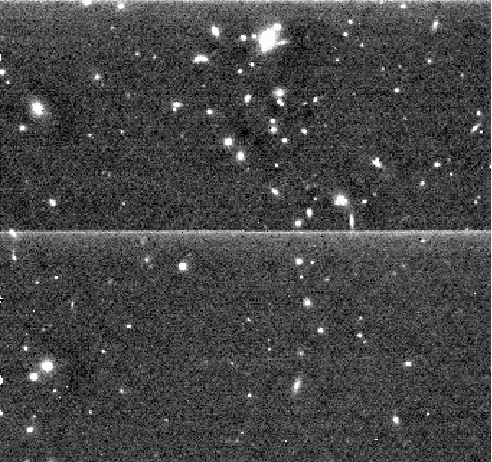
LIRIS@WHT reset anomaly

MOIRCS@SUBARU reset anomaly, before and after correction

10.5.1. Parameters

• DT (optional): The SExtractor detection threshold per pixel, given in units of sigma of the sky background noise. If left empty, no masking will take place.
• DMIN (optional): The minimum number of connected pixels above the detection threshold making up an object. The smaller DT and DMIN, the fainter the objects masked. If left empty, no masking will take place.
• Mask expansion factor: The SExtractor isophotal ellipse is scaled by this number. If set to a number larger (smaller) than 3, the isophotal ellipse will become larger (smaller) than the extent of the detection. This may become necessary if extended low surface brightness objects are present whose extent cannot be detected directly in a single exposure. If you notice that diffuse objects have darker horizontal or vertical bands running through them, then you should consider setting this factor to 6-10, or even more. Otherwise, just leave it empty.
• Store object masks: On by default, so you can inspect the masks and fine-tune DT and DMIN if needed. Background features you want to correct must not be masked.
• Automatic revision of DT: Checks the value of DT. If a larger value is found to yield better results, then the user-supplied value is overridden. Can be tried for correcting an unstable reset anomaly, otherwise should be switched OFF.
• Rejection threshold: A kappa-sigma clipping is performed when calculating average rows/columns. This is the threshold in units of sigma. It should not be chosen too low (lower than 1.5 or 2), in particular if the distribution of background values is non-Gaussian with a bright tail. Check the resulting mask images in MASK_IMAGES to make sure the process is not too zealous.
• Collapse direction: If the brightened feature is horizontal (vertical), select x (y) as the collapse direction. THELI will calculate average columns (rows) in these cases. You can also subtract both horizontal and vertical lines in a single pass (xy). Some HAWAII-2 arrays feature 4 readout quadrants with readout directions rotated by 90 degrees. In these cases you can use either xyyx or yxxy. A small graphical display will visualize the pattern chosen.
• Exclude this region: If an object with a faint extended halo is present in the data, then you must make sure that the halo does not contribute to the measurement area. The halo can be so faint that you do not see it in an individual exposure, and thus it will slightly bias the result. If you stack a large number of images (as is the case with near-IR data), then this can lead to a significant over-correction of the data, visible as a dark horizontal or vertical bar running through the extended source. To avoid this problem, you can define a region that is excluded from the calculation (you must define the left, right, lower and upper boundary in pixel coordinates).