10. SUPERFLATTING
In this section remaining instrumental signatures are removed.
This can either be superflatting, defringing or subtraction
of a background model. For mid-IR data a suitable chop-nod
sky subtraction is offered. Lastly, in order to remove typical
effects such as reset anomalies in near-IR cameras, a collapse
correction can be performed.
If you are unfamiliar with superflatting and defringing, then
please read this
background information first.
10.1. Process SUPERFLAT
This task will take a superflat (as created in the
previous section) and smooth
it with a kernel to obtain the illumination correction (the actual
superflat). The latter is subtracted from the unsmoothed superflat,
yielding the fringe model. You will then have the following images
in your SCIENCE directory:
* SCIENCE_1.fits (the unsmoothed superflat)
* SCIENCE_1_illum.fits (the smoothed version)
* SCIENCE_1_fringe.fits (the fringing model)
10.1.1. Parameters
The following two smoothing options are available:
- Superflat: The value entered here is the size (in pixels) of the
smoothing kernel for the unsmoothed superflat. It defaults to 256.
Values between 100 and 500 appear reasonable.
- Fringes (optional): If the fringing amplitude is low (such as in
optical R-band data), and if the model is calculated from few
exposures only (less than 10-20 images), then one can optionally
smooth the fringing model with a median filter. A value of 1 (2,3...)
means that pixels in a 1 (2,3...) pixel wide border (i.e. the 3x3
(5x5,7x7...) superpixel) are taken into account. Values of 1-2
usually suffice to suppress pixel-to-pixel noise.
10.2. Superflat data
This task divides the flatfielded images by the superflat, i.e.
here you choose the multiplicative superflatting approach.
Filename extension: After running through this step, images have
the character S appended to their filename extension, e.g.
10.2.1. Parameters
- Use unsmoothed SUPERFLAT: Instead of dividing through the smoothed
superflat, SCIENCE_1_illum.fits, the unsmoothed image SCIENCE_1.fits
is used. In some cases this can yield improved pixel-to-pixel noise
in the resulting image as static defects get somewhat suppressed. Has
to be tested from case to case.
- Use OFFTARGET SUPERFLAT: If a blank sky field was observed and
entered in THELI, you will be offered this option (and should probably
accept it).
- Adjust gains: Optionally, THELI can try to correct remaining gain
differences between CCDs of a multi-chip camera, based on residual
gain variations in the superflat. Usually this should not be necessary
as it is taken into account during flat-fielding.
10.3. Defringe data
This step applies the fringe correction image to the data (which
might have been superflatted in the previous step). The fringe image
is rescaled by a correction factor calculated from the ratio of the
modes of the current exposure and the superflat. In other words, THELI
assumes that the amplitude of the fringing scales with the amplitude
of the sky background, which is a valid approach if the sky background
is dominated by airglow.
Filename extension: After running through this step, images have
the character F appended to their filename extension, e.g.
or, if superflatting was performed as well,
10.3.1. Parameters:
- Use OFFTARGET SUPERFLAT: If a blank sky field was observed and
entered in THELI, then the fringing model will be taken from the blank
field.
- Rescale fringe model: If you switch off this setting, then THELI
will not assume that the sky background is not dominated by airglow, but by changing lunar, twilight or zodiacal light
contributions. These components only add to the background level as such,
but do not increase the amplitude of the fringes.
10.4. Subtract SUPERFLAT
This task subtracts the unsmoothed superflat, i.e. it performs an
additive correction. The data will automatically be defringed as well
since the fringing component is still contained in the correction
image. If you observed in the near-IR, this is what you want to do.
Filename extension: After running through this step, images have
the character U appended to their filename extension, e.g.
10.4.1. Parameters:
- Use OFFTARGET SUPERFLAT: If a blank sky field was observed and
entered in THELI, then the background model will be taken from the blank
field.
- Rescale fringe model: You should leave this switch ON.
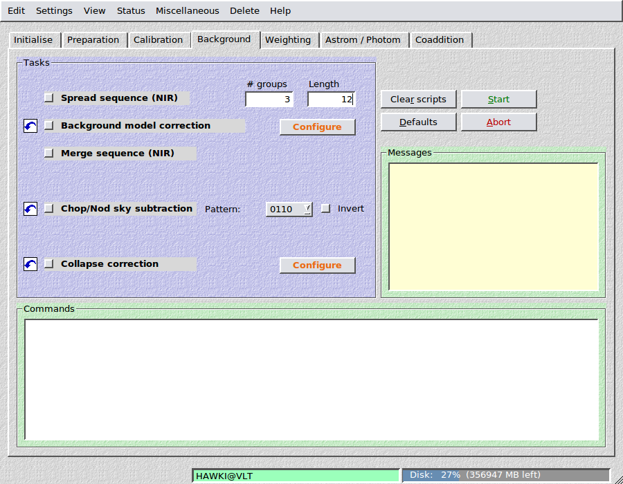
10.5. Chop/nod sky subtraction
This is for mid-infrared data, only. THELI assumes that all science
observations, i.e. on-target AND off-target, resume in the same
directory, and that their alphanumerical order is equivalent to
their temporal order.
You can choose from four different chop-nod patterns, where “1” represents
an image with the target, and “0” an image of a blank sky area. If your
target is very small the chop-nod pattern will not move it off the
detector area, in which case “0” can be considered as another target
observation. Image “0” will be subtracted from image “1” in a pairwise manner.
The available patterns are:
- 0110: 2nd minus 1st, 3rd minus 4th
- 1001: 1st minus 2nd, 4th minus 3rd
- 0101: 2nd minus 1st, 4th minus 3rd
- 1010: 1st minus 2nd, 3rd minus 4th
THELI assumes that this pattern is repeated, i.e. for the pattern
0110 the sequence of exposures is:
0110-0110-0110-0110-...
Invert: If this witch is selected, every second group is reversed, i.e.
for the pattern 0110 the sequence of exposures becomes:
0110-1001-0110-1001-...
Filename extension: After running through this step, images have
the character H appended to their filename extension, e.g.
Note
Images belonging to the “0” chop-nod positions are not present
afterwards anymore. If your source is point-like and also on the detector
for the “0” positions, then they will form a negative image.
10.6. Merge sequence (IR)
At this point one can merge the images again, given one has run the
spread sequence task in the Calibration
section before. The only parameter one has to provide is the number of
groups, which is automatically filled in when the spread sequence task
is executed.
The now fully calibrated exposures in the SCIENCE_Si directories
are merged again in the original SCIENCE directory.
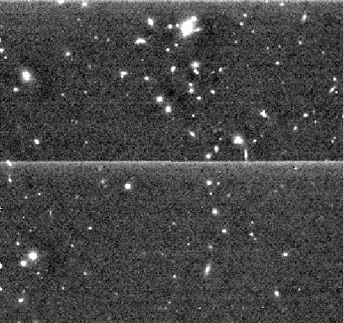
10.7. Collapse correction
If your data exhibits horizontal or vertical linear gradients, such as a
residual reset anomaly in near-infrared detectors, then use this task
to get rid of them. It calculates an average row (or column, or both)
from all rows (or columns, or both) and subtracts it from the latter.
Objects are masked before the average rows/columns are calculated. A
typical reset anomaly would look like this:
10.7.1. Parameters

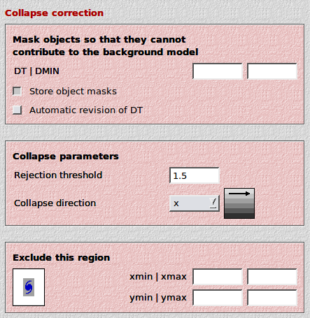
- DT: The SExtractor detection threshold per pixel, given
in units of sigma of the sky background noise.
- DMIN: The minimum number of connected pixels above the detection
threshold making up an object. The smaller DT and DMIN, the
fainter the objects masked.
- Rejection threshold: A kappa-sigma clipping is performed when
calculating average rows/columns. This is the threshold in units
of sigma.
- Collapse direction: If the brightened feature is horizontal (vertical),
select x (y) as the collapse direction. THELI will calculate average
columns (rows) in these cases. You can also subtract both horizontal and
vertical lines in a single pass (xy). Some HAWAII-2 arrays feature
4 readout quadrants with readout directions rotated by 90 degrees. In these
cases you can use either xyyx or yxxy.
- Automatic revision of DT: Checks the value of DT. If a larger
value is found to yield better results, then the user-supplied value
is overridden. Can be tried for correcting an unstable reset anomaly,
otherwise should be switched OFF.
- What to do with the mask:
- Do not store mask: If you just want to collapse correct the images
and move on.
- Mask the input image: This will overlay the object mask over the
input (i.e. uncorrected) image, such that you have a better idea of
the effect of various detection thresholds. Use that to fine-tune
your masking if needed.
- Mask OFC image (2-pass IR skysub): This will overlay the object
mask over the OFC image (if present in a OFC_IMAGES subdirectory).
These masks can then be re-used for a two-pass sky subtraction
(simply restore the OFC images from the OFC_IMAGES subdirectory,
and re-create the sky background model / superflat). The improved
masks will then be used.
- Exclude this region: If an object with a faint extended halo is
present in the data, then you must make sure that the halo does not
contribute to the measurement area. The halo can be so faint that you
do not see it in an individual exposure, and thus it will slightly bias
the result. If you stack a large number of images (as is the case with
near-infrared data), then this can lead to a significant over-correction
of the data, visible as a dark horizontal or vertical bar running through
the extended source. To avoid this problem, you can define a region that is
excluded from the calculation (you must define the left, right, lower and
upper boundary in pixel coordinates).