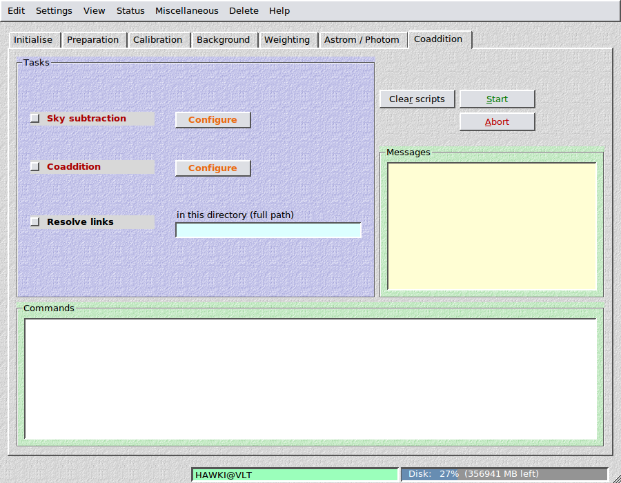
13. COADDITION
This section comprises the final sky subtraction and the coaddition.
13.1. Sky subtraction
This step is generally considered to be mandatory, at least for multi-chip cameras, as otherwise the gaps between the chips show up as discrete jumps in the background (if the latter was variable). If you prefer not to do subtract the sky, then simply omit this step.
Sky modelling has to be done with care if very large objects are present in the field. THELI offers different and very flexible modes for sky subtraction.
Filename extension: After running through this step, images have the string .sub appended to their filename extension, e.g.
NGC1234_1OFC.sub.fits
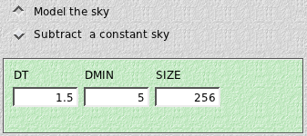
13.1.1. Model the sky
Automatic sky modelling is the default method and useful for all exposures where the largest object is significantly smaller than the field of view of the detector.
Warning
Do not use automatic modelling if you are interested in very faint and extended structures that are not or just barely visible in a single exposure. They will not be masked, therefore enter the background model and as a result will be removed from the data. Subtract a constant sky in this case.
In a first pass, SExtractor is run to remove all objects from the image. The resulting gaps in the field are filled in with a dynamically variable estimate, after which a convolution with a Gaussian kernel is performed. You must provide the usual detection threshold, minimum number of connected pixels, and the FWHM (pixels) of the Gaussian kernel. Optionally, the created sky model can be saved.
Parameters

- DT: This is the SExtractor detection threshold per pixel, given in units of sigma of the sky background noise.
- DMIN: The minimum number of connected pixels above the detection threshold making up an object. The smaller DT and DMIN, the fainter the objects masked.
- FWHM: The FWHM of the Gaussian convolution kernel for the sky background. If you want to remove background features with a linear extent n (in pixels), then you should set this parameter the same or a smaller value. Values less than about 60 do not make much sense.
13.1.2. Subtract a constant sky
A constant sky value should be subtracted if very extended targets are present that prevent the sky from being modelled at the target’s position.
If desired, you can manually fine-tune the estimates for each image. This approach is useful if the target is in size comparable or even larger than the field of view, or if extended very low surface brightness objects are observed which might be mistaken as a background feature and removed by sky modelling.
Parameters
The configuration is split in three parts, not all of them have to be filled in:
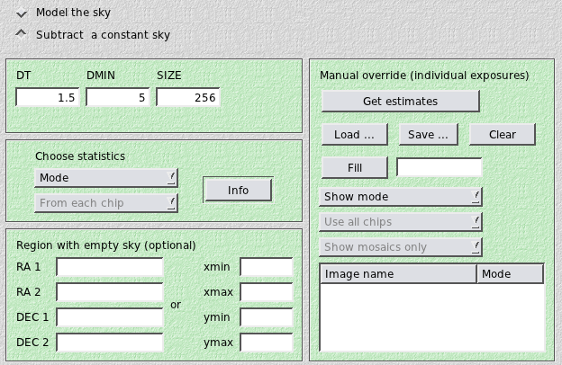
1. Choose statistics
Define how the sky background estimate is determined. Choose between
- Mode: the most common value in the smoothed distribution of pixel values
- Median: the median of the distribution, more stable against outliers than the mean
- Mean: the mean of the distribution
- Lower quartile: the lower quartile of the distribution. Useful if you are not sure about the contamination of some faint extended object.
Mode or median are the best choices in most cases. The other two are unlikely to yield better results.
From each chip: If you are using a multi-chip camera, measure the sky independently in all CCDs.
From chip i: Alternatively, estimate the background from one chip only where you think the sky is representative for the entire mosaic, and subtract this value from all other chips. In this case you can make use of windowing (see below).
Note
This task DOES run SExtractor over the images, using the detection thresholds provided under Model the sky. The statistical estimates are obtained from the object-subtracted images. If you do not provide thresholds, default values will be used (DT=1.5, DMIN=5).
2. Region with empty sky (optional)
You can specify a small window that does not contain any flux from extended objects and obtain the sky estimate from it. There are two options:
- Window fixed on the sky: By entering min and max RA and DEC values, define a window on the sky from which the background is determined. For example, this could be a small dark cloud superimposed on brighter nebulosity. This task also works if the window falls partially into a gap between chips of a multi-chip camera as a consequence of dithering. If no sky could be obtained because the window falls entirely into a gap, then an error message is returned. Click on the update header button in the astrometry section before running this task. In this way you make sure that no differential WCS offsets are present in the header and the window will be centred on the same spot on the sky in all exposures.
- Window fixed on the chip: By entering Cartesian xmin xmax ymin ymax chip coordinates, the window from which the sky is estimated is always taken from exactly the same detector area, independent of any dither pattern. This task is only meaningful for multi-chip cameras if the sky is estimated from a single chip only.
If you leave one or more of the fields empty, the entire detector area will be used.
3. Manual override (optional)
Use this feature only if you want to manually fine-tune individual sky background values.
Note
This task DOES NOT run SExtractor to remove objects from the images, the thresholds given under Model the sky are not applied. The statistical estimates are obtained from the images as they are.
The following settings can be made:
Get estimates: Determines from each image (no objects subtracted) the mode, median, mean and lower quartile. If a window was defined, the sky will be estimated from it. This has to be done only once, as the output is stored internally. The result will be shown in the table, one value for each image. The numeric values are editable. This task will always run on all chips, no matter what selection you make elsewhere.
Load/Save: The statistics obtained by Get estimates is saved in:
SCIENCE/skybackground_xxx.stat.
You can Load such a statistics if it already exists, or Save it under a particular filename. You do not need to save the table explicitly. THELI will use the values displayed in the table when you leave this dialog (the what you see is what you get principle).
Fill: Replaces any value in the table with the numeric value entered in the field to its right. This does not erase the values obtained through Get estimates. If you select e.g. Mode again for the display, the previous values will be restored. This button can be clicked instead of Get estimates at the very beginning, for example if you know that you only want to subtract a value of e.g. 587.3 from all images.
Show mode: Can be used to display either the mode, the median, the mean or the lower quartile in the table. You can cycle through the various measures without loosing data.
Use all chips: If you have data from a multi-chip camera, select whether the sky value displayed is taken from each chip individually, or only from a particular chip whose background you consider representative for all other chips. For example, all 8 CCDs of the camera cover a large object, and only chip no. 5 contains a small region with empty sky. Then you would define the window, click on Get estimates and select Use chip 5. You can cycle through the various chips without loosing data.
Show mosaics only: Allows you to display exposures only, i.e. the table will contain only one line for a group of n images, where n is the number of chips in your camera. The name of the image of the first chip will be displayed, representative for all other images of the same exposure. The other option is to show all images of all chips.
WYSIWYG principle for constant sky configuration
When you close the dialog, sky subtraction will be performed according to your settings. If you manually fine-tuned the sky, the content of the table will be saved to
SCIENCE/skybackground.use
together with the associated image names. If a file with the same name is present already, it will be overwritten without warning. This file will be read once you launch the sky subtraction. If you selected Show mosaics only, then all images of one exposure have the same sky value assigned. That is, what you see is what you get.
13.2. Coaddition
This last step is internally broken down into several other steps. First, images are resampled to a common output grid taking into account the astrometric solution obtained previously. This step is parallelised. In an optional second step the resampled pixels contributing to one output pixel are compared and outliers can be rejected (their weight is set to zero). This task is not (yet) parallelised and can be lengthy for larger mosaics. Afterwards, the resampled images are combined into the coadded image, and the header of the latter is updated with various parameters and measurements. Resampling and stacking are done with Swarp.
The coadded image can be found under
SCIENCE/coadd_xxxx/coadd.fits

SCIENCE/coadd_xxxx/coadd.weight.fits
where xxxx stands for an unambiguous, user-provided identifier. Thus different coadditions can be created without overwriting older stacks.
13.2.1. Parameters
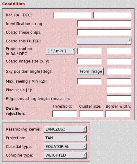
- Reference RA / DEC: The reference coordinates for the projection on sky. You can leave them empty, in which case they will be determined automatically. However, if you have data of the same target taken in different filters, you should use identical values for all coadditions. You MUST use identical values if you plan to create a color picture or to do difference imaging. The reference coordinates should not be too close the border of the image as otherwise the coadded image might be truncated.
- Identification string: This string will be appended to the name of the coadd directory. Therefore different coadditions can be made without overwriting each other. If left empty, it is set to default.
- Coadd these chips: For a multi-chip camera you can choose to coadd only certain chips instead of all of them. If left empty, all chips will be stacked.
- Coadd this FILTER: If you run the astrometry over images taken in different filters, then these will be mixed in the SCIENCE directory. Tell THELI here which filter it should stack. You do not need to move images taken in other filters to parking directories.
Proper motion: If you observed moving targets, you can enter here the proper motion vector. THELI will look up the DATE-OBS keyword in the FITS header and apply a linear offset to the WCS solution contained in the astrometric header. Like that the moving target will fall on top of itself in the coadded image instead of leaving a trail:
Good if you want to detect e.g. faint TNOs not visible in single exposures.
- Coadd image size (x,y): For very wide fields of view and all-sky projections, the size of the output image is difficult to predict automatically. It many such cases it will be too small, and you can provide the output image size in pixels manually. You can estimate the size in pixels as follows, for both axes: field of view in degrees divided by pixel scale in degrees, and add some margin for good measure.
Pixel scale: The pixel scale of the output image. You can decrease or increase the resolution. The latter only makes sense if your data is undersampled and if you have a sufficiently large number of dithered exposures, or if you want to match your image to that taken with another telescope or camera. Upsampling by more than 50% is rarely useful with ground-based data.
Note
If left empty, the native pixel scale given in the instrument configuration will be used. For instruments with exchangable foreoptics (e.g. SOI@SOAR, FORS1+2@VLT) this is the most frequently used pixel scale.
Sky position angle: If left empty then THELI will orient the coadded image such that North is up and East is left. If you want a different sky position angle, then enter it here (counted positive from North over East). If your data was taken under a (unknown) non-zero position angle, you can estimate it by clicking on the From image button. This will not rotate your images into standard orientation. However, note that a flipping of axes will always be corrected.
- Edge smoothing length: Mosaic data of very extended targets often cannot be fully sky-subtracted as there is no way to estimate the real background level without blank field exposures. In this case one usually subtracts a constant value, which can lead to small discontinuities in the overlap areas. By smoothly reducing the weight map at its borders to zero these transition areas can be blended into each other, eliminating the discrete jumps while preserving photometry. The value entered is the width of the softened edge. As a rule of thumb, it should approximately be the same as or smaller than the extent of the overlap in pixels (for example 50 to 100).
- Maximum image seeing: If you want to exclude images with a seeing above a certain threshold, then enter this value here.
- Minimum relative zeropoint: If you want to exclude images with a relative zeropoint worse than this threshold, enter it here. The relative zeropoints are normalised such that their mean is zero. Images with worse transparency have negative values, images with better transparency have positive values.
Outlier rejection threshold: The clipping threshold in units of sigma. If a (resampled) pixel deviates by more than this from the mean value of resampled pixels at this location, then it will be removed from the stack (i.e. it has its weight set to zero). If left empty, no rejection will be performed.
A value smaller than 4 should only be used if you have 15-20 exposures or more, ideally with a cluster size larger than 1 (see below). Values less than 3 hardly make sense. If you feel you need such aggressive rejection, probably something else went wrong in your data reduction process, such as mismatched darks, bad sky subtraction (near-IR only), or you forgot to dither your telescope. A warning message will be shown.
Outlier rejection cluster size: Only mask pixel groups consisting of that many bad pixels above the threshold. If you find that masking is too zealous, then increase this to values larger than 1. Values larger than 9 are not permitted and will be reset to 9. Requires the rejection threshold to be non-empty. For the Lanczos2/3 kernels values of 3-6 work appear plausible.
Outlier rejection border width: If a pixel is found to be bad, then also mask a ring of pixels around it. This parameter specifies the width of this ring in pixels. Requires the rejection threshold to be non-empty.
Resampling kernel: Choose from
- Nearest neighbour (NN): No resampling (flux distribution between output pixels) is done. Leads to significant astrometrical artifacts.
- BILINEAR: Use only for extremely undersampled images
- LANCZOS2: Use for significantly undersampled images
- LANCZOS3: Optimal for well-sampled images. If you notice dark edges in your star profiles, then you are likely undersampled and should go with LANCZOS2 instead.
- LANCZOS4: Best from a sampling point of view, but leaves large artifacts around hot pixels and other steep image features. Slow.
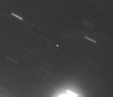
Animation of images resampled with LANCZOS3 (top) and NN (bottom) kernels.
Note the erratic wiggling of stellar positions using the NN kernel:

The NN kernel can also lead to significant distortions within the PSF, depending where on the pixel grid a source is projected. Look at the bright star immediately above the diffuse large galaxy. In one of the images it appears significantly elongated, whereas this is absent with the LANCZOS3 kernel.
- Projection type: Use your preferred projection type. Will only make a difference for fields of view larger than several degrees. For a complete list and more explanations see below.
- Celestial type: The coordinate system into which you want to project
your images:
- NATIVE: use whatever is defined in the FITS header. In case of THELI this will be EQUATORIAL.
- EQUATORIAL: the classic RA and DEC sky coordinates
- GALACTIC: galactic coordinates
- SUPERGALACTIC: supergalactic coordinates
- ECLIPTIC: useful for solar system stuff
- Combine type: How the resampled images are combined:
- WEIGHTED: yields the best S/N
- AVERAGE: better S/N than MEDIAN but sensitive to outliers
- MEDIAN: worse S/N than AVERAGE but stable against outliers
- MIN: use the smallest pixel value in the stack
- MAX: use the highest pixel value in the stack
- CHI2: uses chi-square for the stack (all pixel values will be non-negative)
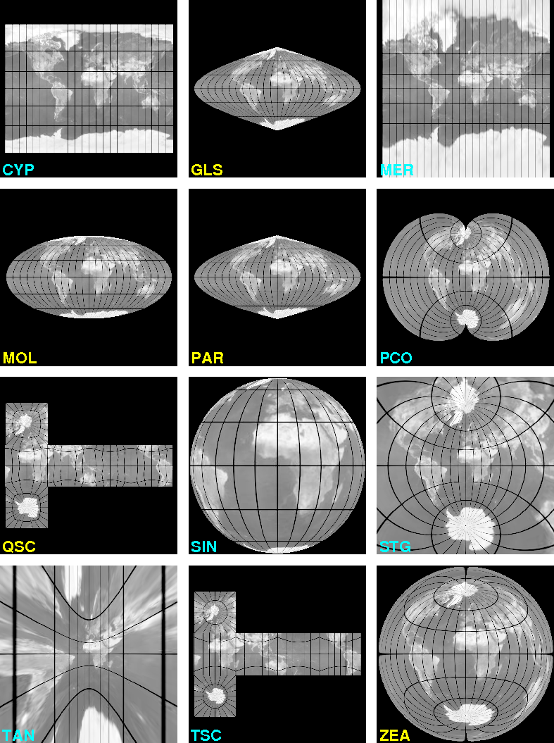
13.2.2. Sky projections
The projections of the proposed FITS WCS standard are available in THELI (copied from the SWarp manual, thanks Emmanuel!). Nine of them are equal-area projections, i.e. they preserve surface brightness (indicated with yellow labels).
Which of the projections is chosen does not really matter as long as the field of view is about less than 10 degrees. For larger fields projection effects become significant.

Zenithal projections
- AZP: Zenithal perspective
- TAN: Distorted tangential
- STG: Stereographic
- SIN: Slant orthographic
- ARC: Zenithal equidistant
- ZPN: Zenithal polynomial
- ZEA: Zenithal equal-area
- AIR: Airy
Cylindrical projections
- CYP: Cylindrical perspective
- CEA: Cylindrical equal-area
- CAR: Plate carree
- MER: Mercator
Conic projections
- COP: Conic perspective
- COE: Conic equal-area
- COD: Conic equidistant
- COO: Conic orthomorphic
Pseudoconic and polyconic projections
- BON: Bonne’s equal-area
- PCO: Polyconic
Pseudocylindrical projections
- GLS: Global sinusoidal (Sanson-Flamsteed)
- PAR: Parabolic
- MOL: Mollweide
- AIT: Hammer-Aitoff
Quad-cube projections
- TSC: Tangential spherical cube
- CSC: COBE quadrilateralized spherical cube
- QSC: Quadrilateralized spherical cube
Note
Some projections require additional PVi_j parameters in the header, i.e. you must run Scamp with distort>1:
CYP, CEA, COD, COE, COO, COP, BON
13.3. Resolve links
If you spread the images of a multi-chip camera over several hard disks under Create links, then you can recollect them in their main directory (the one where the links are). Just enter the name of the directory where you want to resolve the link structure.