14. Miscellaneous THELI modules

THELI offers a few additional tasks you can run outside the framework of the main reduction thread.

14.1. Combine images

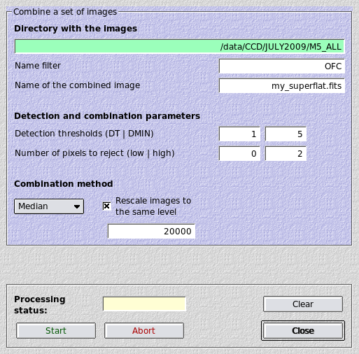
Combine a set of arbitrary images in a given directory (without taking into account image shifts etc). Images are stacked as they are.

14.1.1. Parameters

• Name filter: This should be the status string between the chip number and the file suffix, for example OFC. If left empty, all images in the directory will be combined. Separate stacks will be created for multi-chip camera data.
• Name of the combined image: If left empty, the combined image will have the name of the directory. For example, if the images are in a directory called NGC1234, the stacks will be called NGC1234_i.fits where i is the chip number.
• DT/DMIN: Objects will be removed from the images using SExtractor before combination takes place. These are the detection threshold per pixel above the sky noise and the minimum number of connected pixels above this threshold forming an object. If these fields are left empty, then objects are left unmasked.
• Number of pixels to reject: The number of lowest and highest pixels in the stack to be rejected.
• Combination method: Choose between median and mean.
• Rescale images: Optionally, images can be rescaled to the same background level before combination. That could be useful e.g. for the creation of a superflat.

14.2. Imalyzer (image analysis)

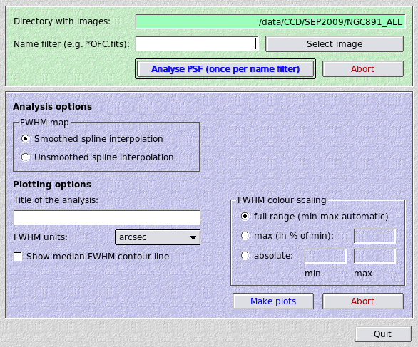
If your individual exposures (per chip) contain about 100 stars or more, a more detailed image analysis using THELI’s Imalyzer can be performed. It automatically extracts stellar sources and performs a very sensitive weak-lensing style PSF analysis. FWHM variations across the detector areas are modelled using a 2-dimensional spline fit. The PSF anisotropy (ellipticity) is displayed as a stick plot superimposed over the FWHM map.

The anisotropy is calculated from the second brightness moments of the object’s filtered flux distribution. In the idealised case of a star with an elliptical Gaussian brightness distribution, the ellipticity e is reduced to

where a and b are the major and minor axes. This should simply serve for illustration purposes, as in general stellar profiles are very different. In the moment description, a perfectly round source has an ellipticity of 0, and a highly elliptical one will be close to 1.

14.2.1. Parameters

• Name filter: The Imalyzer will process all images in a given directory, unless a name filter such as ngc1234_night1_*OFC.fits is provided. You can also enter here the name of one individual image.
• Title of the analysis: You can specify an unambiguous string which will serve as a title for the analysis. In this way you can run Imalyzer with different configuration settings without overwriting previous results.
• Smoothed spline interpolation: Applies a strong smoothing to the FWHM field during spline interpolation. The result is more idealised and representative for what the optics delivers.
• Unsmoothed spline interpolation: Only a minimum of smoothing is applied to the data field before spline interpolation, in order to reject outliers.
• Show median FWHM contour line: Overplots a thick white line indicating the median level of the FWHM map.
• FWHM units:
  • arcsec: The FWHM map will be displayed in units of arcseconds
  • pixel: The FWHM map will be displayed in units of pixels
  • minFWHM: The FWHM map will be normalised to the smallest FWHM, i.e. this is a relative scaling as compared to the previous two.
• FWHM color scaling:
  • Full range: For each image the min and max FWHM are determined, and the full color range will be used for display. Images are treated independently of each other.
  • max (in % of min): If set to a numeric value of e.g. 50, the upper FWHM limit shown will be 50% larger than the smallest one. Images are treated independently of each other.
  • absolute: The lowest and highest FWHM shown. This is the same for all images. Units are either in arcsec or pixels, depending on which ones you chose for the display.

14.2.2. How to run Imalyzer

Imalyzer requires that you run the Create source cat task first.

Select the directory and optionally a subset of images, then click on Analyse PSF. This has only be done once for that particular set of images. It will create a sub-directory called

SCIENCE/cat/ksb/

in which the PSF analysis results are stored per image. Once done, set your plotting options and click on Make plots. This will do the FWHM spline fit and also read the output from the PSF ellipticity analysis for the stick plot.

Results are collected in an interactive html file (example) which is automatically displayed provided you have ‘firefox’ installed. If you use a different browser, point it to

SCIENCE/imagequality/<yourtitle>.html

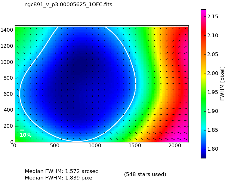
14.2.3. Interpreting Imalyzer results

With several hundred stars the Imalyzer results should be fairly robust. Given that no polynomials are used in the FWHM fit, it represents the actual FWHM variations measured, albeit smoothed on a scale on which FWHM variations appear plausible. The ellipticity indicated is a blend of individual data and an iterative fit.

• With well-aligned optics the area of lowest FWHM should appear close to the centre of the image (or the optical axis), which might be outside the currently investigated chip. If this is not the case, then probably something is misaligned, or the FWHM variations are so small that the variations indicated are negligible. If the plot is clearly skewed, then chances are that there is something misaligned. This could either be the optics, or a tilt of the CCD with respect to the focal plane, or else.
• Ellipticity and FHWM can be correlated: If something is misaligned in the optics, then then the PSF e.g. becomes more elliptical in the corners of the field (and therefore the FWHM measured rises, too). It can also work the other way round: if for example the seeing increases, the PSF gets rounder as optical imperfections are blurred. Likewise, if the seeing gets better, the PSF reveals more imperfections. With undersampled data the PSF can become quite elliptical, but since it is so compact this might very well be of no importance for your scientific purposes.
• With significantly undersampled data the accurate determination of FWHM and ellipticity can be unstable. Imagine a perfectly round PSF with a FWHM comparable to one pixel. If the star falls right on the boundary between two pixels, it will essentially appear twice as long as broad and the FWHM will be artificially increased, compared to the situation where the star falls onto the centre of a pixel.

Therefore, when interpreting Imalyzer results, you should always take both FWHM and ellipticity into account. Don’t forget to look at the color scale bar indicating the FWHM range displayed, in particular if one of the two non-absolute scalings was chosen. Knowing the observing conditions and the telescope also helps.

For example, a slow change in optical alignment with increasing zenith distance will result in a slowly drifting FWHM pattern, whereas optical realignment between exposures shows up as a sudden jump. In images which short exposure times the FWHM map may be misleading as seeing variations can cause noticeable distortions. Or in a closed tube assembly rising warm air on one side of the tube can lead to increased FWHM in some part of the image, mimicking a tilt of the CCD.

14.3. Image statistics

This module tabulates basic image properties and displays some of them graphically:

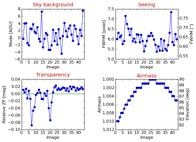
14.3.1. Parameters

• Name filter: The statistics module will process all images in a given directory, unless a name filter such as ngc1234_night1_*OFC.fits is provided. You can also enter here the name of one individual image.
• Area for background estimation: Use these 4 fields to define an area of empty sky should the rest of the detector be covered by an extended source.
• FWHM and HFD units: Whether you want the FWHM and the HFD (half flux diameter) displayed in pixels or arcseconds.

14.4. Absolute photometric ZP

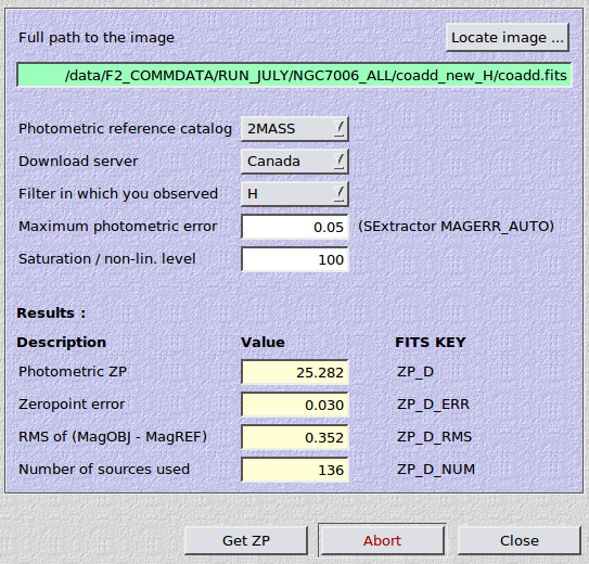
This module can be used to obtain a crude absolute photometric zeropoint for an image, provided that you observed in similar passbands (either ugriz or JHKs). The image must have a valid WCS solution in the FITS header. The method used is essentially the same as the direct photometric calibration in the main reduction framework.

THELI will return:

• the zeropoint for the exposure normalised to an integration time of 1s, written to a ZP_D keyword
• the zeropoint error (ZP_D_ERR)
• the rms scattering between objects in the image and those in the reference catalogue (ZP_D_RMS)
• the number of sources that went into the fit (ZP_D_NUM)

14.4.1. Parameters

• Photometric reference catalogue: SDSS or MASS
• Download server: Switch between different servers should one of them not respond
• Filter in which you observed: Either one of ugriz or one of JHKs
• Maximum photometric error: Only sources with a SExtractor magnitude error equal to or less than this value will enter the fit.
• Saturation / non-lin. level: Objects containing pixels in the coadded image with a value higher than this threshold will be excluded from the analysis. This can be used either as a saturation or a non-linearity threshold.

Warning

This approach does not take into account color terms arising from different total throughput curves between your telescope/filter/camera combination and the one used for SDSS or 2MASS. If you need absolute zeropoints better than about 0.1 mag then you should consider fine-tuning the ZPs using a comparison of instrumental stellar tracks against those in the Pickels library, or a classical approach based on standard star observations.

14.5. Animate

The resampled images created during coaddition have accurate WCS information in their headers and can therefore be animated to check for moving or variable objects. THELI will create animated GIFs from the data and stores them as

SCIENCE/coadd_xxx/movie/anim_i-j.gif

Examples, with and without proper motion vector during coaddition (left, respectively right):

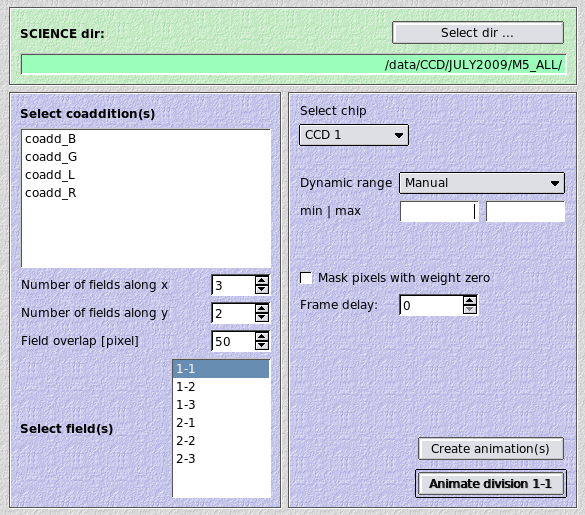
14.5.1. Parameters

• Select coadditions: After entering a SCIENCE directory, you will be presented with a list of the coaddition directories found. You can select either one or several.
• Number of fields along x|y: One usually does not want to to produce a full-scale animated GIF, but concentrate on smaller sections. These two parameters control into how many sections the image is split along x- and y-directions. Counting starts at the lower left. For example, if you set x=3 and y=2, then the field labelled 2-3 would correspond to the third image from the left, in the second row from the bottom.
• Field overlap: This is the overlap in pixels between fields.
• Select field(s): Choose here for which field(s) you want to create or display an animation.
• Select chip: For multi-chip cameras, you must specify from which chip the resampled images should be taken. This option is not visible for single-chip cameras.
• Dynamic range: The animated GIF has a dynamic range of 8 bit, only. Therefore you must select which range should be displayed. Two options are available:
  • Manual: Enter min and max levels (black- and white-point) for the GIFs. Since images are sky-subtracted, min should be negative and max positive, the latter with an absolute value about 5 times larger than min. For example, min=-100 and max=500.
  • Automatic: Will apply a ds9-style automatic z-scale range. You can adjust the contrast value from -9 to +9.
• Mask pixels with weight zero: Pixels which have a value of zero will be masked (set to zero) in the resampled image. If your data has a lot of hot pixels, you can suppress them in this manner in the animated GIF.
• Frame delay: The delay between images in the animated GIF in units of 1/10th of a second. Note that this delay is ignored by the Animate field button which simply displays the images as rapidly as possible (it does not load the animated GIF but the individual frames)
• Create animation(s): Creates animated GIFs for all selected fields
• Animate field: Shows the animation for the currently selected field. Note that the frame delay is ignored by this function.