15. Near-infrared data
While near-infrared detectors are fundamentally different than CCDs, the general data reduction steps required are essentially the same. Therefore, once you understood how to reduce optical data with THELI, you already have most of the knowledge required for the near-IR regime. However, instrumental and atmospheric effects make reduction of near-IR data tricky. The sections below summarise how you deal with this in THELI.
15.1. Crosstalk
Crosstalk can in general be corrected well, provided that it is spatially stable. The latter is not always the case for near-IR detector arrays. In particular recent HAWAII2 sensors with multiple parallel readout sections can show crosstalk in form of compact positive and negative ghost images whose amplitude varies between readout sections. THELI assumes that the amplitude is the same, therefore the correction will only partially remove the effect (if at all). If you know in advance that this will be a problem for your science case, then consider choosing different camera rotator angles for your observations.
15.2. Reset anomaly and imaging equilibrium
Some detectors will exhibit a horizontal or vertical brightening towards one edge of the readout quadrant. It is unstable and in general depends on temperature, exposure time, the number of previously executed exposures, and can also have an erratic component. You can correct for it using the Collapse correction.
In very rare cases, such as for LIRIS@WHT (the only one the author is currently aware of), another problem occurs. If you take n exposures at a certain dither point and then move on to the next dither point where you repeat the same n exposures, piece-wise background correction can become necessary. In other words, even if the physical sky background does not change, the instrumental background pattern can change in a repeated fashion: it is the same for all k-th exposures in the series, but different from the pattern inherent to all (k+1)-th exposures (and so on). To apply such a group-wise background correction, use the spread sequence task and then proceed as normal. THELI will take care of the rest.
15.3. Sky background
15.3.1. Characteristics
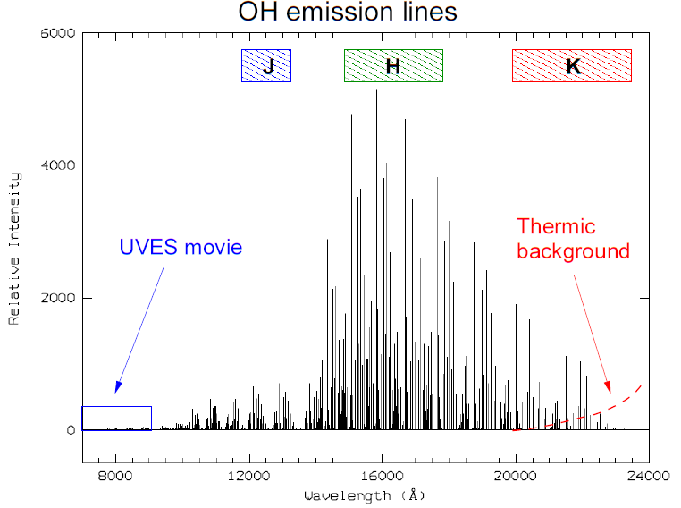
Optical and near-infrared imaging differ most when it comes to atmospheric sky background. In the near-IR the background level changes on time scales of a few minutes, and on angular scales of a few arcminutes. Some nights are very stable and one can calculate a single static background model that will suit all exposures taken within a e.g. 20 minute window. Other nights will be highly unstable and it is necessary to create individual background models for each exposure (dynamic modelling). More about dynamic and static models can be found here.
In general, H-band is affected most by this highly variable airglow, as shown by this night sky spectrum:
15.3.2. Exposure times
Exposure times in near-infrared imaging are rather short, for two reasons:
- The background is variable: Frequent dithering is necessary to achieve good background subtraction.
- The background is high: Exposure times must be short to avoid non-linearity or object saturation.
The following table contains typical night sky surface brightnesses in mag/sq. arcsec, and characteristic exposure times for detectors with 0.1-0.2 arcsec/pixel scale. Integration times for Z are for near-IR detectors, for optical detectors they are usually longer (optical and near-IR Z-band filter curves are not necessarily identical):
| FILTER | B | V | R | I | Z | J | H | Ks |
|---|---|---|---|---|---|---|---|---|
| Surface brightness | 22.7 | 21.9 | 21.0 | 20.0 | 19.0 | 16.0 | 14.5 | 13.5 |
| Exposure time [s] | 600 | 600 | 300 | 300 | 60 | 30 | 20 | 10 |
Narrow-band filters
Exposure times with near-IR narrow-band filters should be kept as short as possible, and made as long as necessary in order to reach background limited images. There is a trade-off depending on which narrow-band filter you are using. Exposure times up to 300s are possible for filters where less airglow is present.
Co-averaging, or co-addition
One problem due to short exposure times in the near-infrared is that for high-galactic latitude fields the number density of discernible sources can become very low. This can be critical from an astrometric and photometric point of view, as internal data calibration is difficult. Most observatories offer the possibility to average a sequence of k exposures on-chip before the image is read out. In this manner the S/N is improved without running into problems with non-linearity, saturation or the 16bit dynamic range. This process is sometimes called co-averaging (or co-adding, depending on the implementation), the individual integration time is called DIT, and the number of co-averaged or co-added exposures NDIT.
15.4. Background modelling
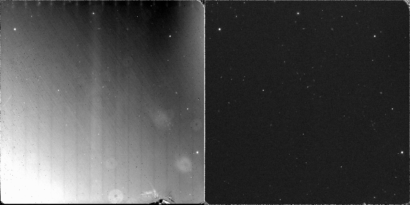
When you reduce near-IR data the first time, you’ll probably be surprised that after flat-fielding the image appears everything else than flat. The amplitudes of the residual background variations from sky and instrumental contributions are usually much larger than the fluxes from astrophysical objects. Frequently, you won’t even be able to discern any objects at all in the data after flat-fielding.
The following example displays a 6x10s exposure (DIT=10, NDIT=6) taken with one of the four 2kx2k detectors of HAWKI@VLT in Ks-band. Shown in the left panel is the appearance after flat-fielding, and the right panel displays the same image after subtraction of a (dynamic) background model:
15.4.1. 1-pass modelling
Which background model is most suitable for the data does not only depend on the atmosphere, but also on the target. If the field is sparse and contains point sources only, then very often a simple (static or dynamic) background model with basic min-max rejection and median combination is sufficient. Leave the DT, DMIN and SIZE thresholds empty.
If the field is crowded and you have many exposures, switching on additional object masking can avoid the background model to be biased by object fluxes. Use some explicit settings for the SExtractor detection thresholds, e.g. DT=10 and DMIN=10. Thresholds must be chosen high enough such that no background features are masked. The mask images are called *OFC.mask.fits and are collected under
SCIENCE/MASK_IMAGES
once processing is finished. You should eyeball them and see if sky features were detected. In addition, you can use min-max rejection as outlined above.
15.4.2. Iterative or 2-pass modelling
The main problem with the 1-pass approach just outlined is that good object masks can only be created from a flat image. This is particularly important if the field contains extended sources, parts of which are too faint to be visible in the flat-fielded exposures. If this hidden flux is not masked, the background model will be biased, leading to significant over-subtraction. Very often this will only be visible in the coadded image, showing up as dark areas or patches scattered around brighter sources. In such cases an iterative approach is advisable:
Create the static or dynamic model as normal. You can safely switch off object masking by leaving the DT and DMIN parameter fields empty.
If you chose a static (dynamic) background model, set the window size to a zero (non-zero) value. In both cases rescale the model.
Once THELI has finished, your images will have the status string OFCB written into their file names and should look very close to flat (if no iterative modelling is required you can leave here and jump to the weighting process). The following sub-directories are now in the SCIENCE directory:
SCIENCE/SPLIT_IMAGES
SCIENCE/OFC_IMAGES
SCIENCE/MASK_IMAGES
The first contains the raw data after splitting. The second contains the flat-fielded (and possibly dark-subtracted exposures), and the last one contains the mask images.
Repeat step 1, but this time set DT and DMIN to their default values to trigger object masking. THELI will recognise that the task is run a second time (due to the presence of OFCB images). In this case the object detection will take place on the temporary OFCB images with good background, and the corresponding pixels will be masked in the original, flat-fielded only OFC images. The newly created mask images from these data are then also applied to the OFC images, resulting in a new batch of OFCB exposures. The previous ones will be kept in a OFCB_IMAGES_1PASS directory for comparison.
The process is straight forward and should provide you with fairly flat images.
15.4.3. Using separate blank SKY exposures
If your targets are really extended and/or very faint, then you should seriously consider observing blank SKY fields. They will be automatically used in the correct manner once collected in a separate directory and defined in the Initialise section. No additional settings have to be made. You should check though that the images have correct MJD-OBS header keys after splitting.